3.1. The Method of the Growth Factors
3.1.1. Summary
To satisfy a wide variety of patients with a series of mass-produced stems, it is necessary to take into account the anatomical variations having largely independent causes and very different amplitudes, such as for example the length of the femur depending above all on the size of the patient and the internal diameter of the medullary canal which varies especially with the age and the activity of the patient.
To obtain this result, the dimensions of the prosthesis (width, length, thickness), the dimensions of the neck (length, diameter), grow regularly from one size to the next, with values defined independently of each other and in percentage for each dimension.
It is these multiplicative factors (similar to interest rates) that I have called since 1981 "Factors of Growth" or "Growing Factors" or "GF".
3.1.2. The Growth Factors
Growth Factors are the basis of the mathematical method that I specially developed in 1981 to calculate the optimized series of implants. This method also makes it possible to calculate all the sizes of the series simultaneously.
To satisfy a wide variety of patients with stems manufactured in series and not made to measure, it is necessary to take into account anatomical variations, having largely independent causes, and very different amplitudes. For example, the length of the femur, which depends above all on the size of the patient, and the internal diameter of the medullary canal, which varies above all with activity and evolves with age.
The length, the width, the thickness of the prosthesis, the length and the diameter of the neck, must grow regularly from one size to the next to obtain this result. For the series of Optimized Sizes, I vary each dimension, from one size to the next, with values defined in percentage and independent for each dimension.
3.1.3. Simplified examples of the interest of the method
To simplify the explanation, I prefer to restrict myself to lengths, stem widths and neck lengths (other dimensions being less demonstrative).
Take for example a series of sixteen sizes to cover all patients, the sizes of the patients ranging from 1.40 meters to 2 meters.
So from largest to smallest, there is a variation of 1.43, or 43%. This variation is to be distributed over the sixteen sizes of the series. The widths of rods corresponding to the diameters of the medullary canal present, for the same population of patients, values ranging from 6mm to 30mm, i.e. a total variation of a factor of 5, therefore 400%, also to be distributed regularly over the sixteen sizes.
If the length factor of 1.43 was also used to vary the width, we would obtain rods varying far too little in width (for example from 10 to 14 mm) and unusable both for patients with a 6 mm canal only for patients with a 30 mm canal. A truly satisfactory solution to this problem cannot be obtained by dividing the interval linearly between the largest size and the smallest size of each dimension.
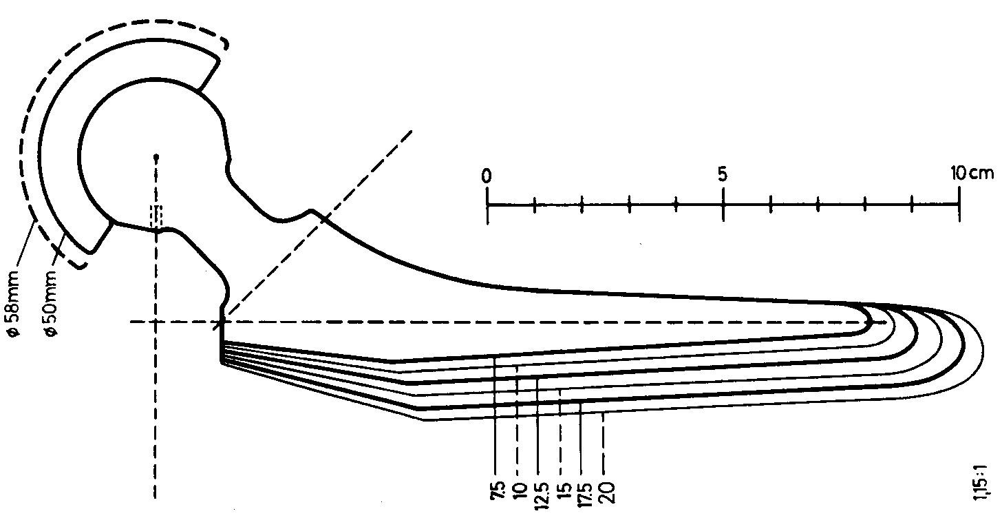
Example of a series of stems before the application of my method. (distal widths of first generation Zweymüller stems, 1979). width 10, 12.5, 15, 17.5, 20. Between 10 and 12.5 the growth is 1.25 or 25%. Between 17.5 and 20 the growth is only 1.14 or 14.3%.
For a patient whose femur would theoretically require a size 12 stem (not available), only a size 10 can be implanted. The patient will have received a prosthesis 20% too small for his femur! It will be badly prosthesed with obvious risk of sinking (this case happened several times in my presence).
On the other hand, for a patient whose femur would have required an ideal size 17 stem, size 15 is available, therefore only 12% too small for his femur. This patient will be "significantly" better equipped than the one in the previous example. The femur of this patient, with a larger bone stock, could have been enlarged by grating without risk to 17.5, which could not have been the case for the small femur in the previous example.
This shows that with a small number of sizes distributed linearly, major differences in conduct are to be observed by the Operator, from one patient to another, and that patients of small size more often receive unsuitable sizes.
There have been so-called "millimetric" prostheses on the market, the large number of which solved the patient's problem fairly well, but the differences between the very large sizes of which were unnecessarily close together, requiring moreover too large a stock.
I therefore looked for a mathematical model allowing all patients, from the smallest to the largest, to have strictly equal chances of receiving the size closest to the ideal size, with a rate of imperfection and uncertainty constant for all patients, and allow the operator to maintain the same behavior for the choice of sizes for all his patients.
I have defined the gap between two successive sizes so that the operator can always grate an extra half size without difficulty, and even a little more if necessary. This is the essential principle of the concept of Optimized Sizes.
3.1.4. Choice of Growth Factors
I first, among all the dimensions of an implant, defined which are the dimensions which must vary from one size to the next, whose logics are independent between them, and which are the dimensions whose logics of variation are linked.
It seemed to me sufficient to include in the calculation process a maximum of 8 different Growth Factors.
1. important factors such as those which govern the width of the shaft, the length of the anchorage zone in the bone, the neck length and the anteroposterior thickness,
2. factors varying the diameter of the neck at the base of the cone and the amplitude of the trochanteric fin,
3. and possibly factors whose usefulness is secondary, for example the diameter of the suture holes and the size of the distal ogives, the variation of which has only an aesthetic role but which gives the series its beautiful impression of continuity .
Some additional factors are made up of the linear combination of two of the previous factors and will be used, for example, to scale the Function of the Distal Ogive.
Each element of the Growth Factors Table is obtained with the successive powers of the Growth Factor chosen to cover the 16 sizes provided. The average size is used as the origin for staggering, both towards the large sizes and towards the small ones. Sizes larger than the average size receive positive powers of the Growth Factor considered, and sizes smaller than the average size receive negative powers.
remplacer peut etre Espace vectoriel à 16 dimensions, pour 4 tailles
In the software, the number of factors and the number of sizes can be extended if necessary.
The detailed description of all the geometry of the implant, common to all sizes of the prosthesis series, is written in the form of a computer program. The program specific to a series of implants contains approximately 4000 instructions. No design software was used to create these implants. Every geometric detail has been formulated mathematically. No approximation, smoothing or automatic curve generator was used.
In my system, the whole series of sizes is calculated simultaneously and the description program includes all the relationships between the successive sizes, whereas for competing prostheses, without exception, the creation is done with assisted drawing software by computer and only one size is worked out at a time, without any formulated and calculated relationship between successive sizes, and the dimensions are defined and entered manually.
3.1.5. The system uses some properties of vector spaces
Instead of calculating a series of three-dimensional sizes in an ordinary orthonormal space, in which the vectors perpendicular to each other, on the X, Y and Z axis, have the length of the unit of measurement used ( the millimeter by example), I compute the series of Optimized Sizes in an 8-dimensional vector space for each size. The 16 powers of each growth factor define sixteen collinear vectors of different length. The 8 growth factors can be associated with 8 different directions in space, some of them perpendicular to each other and others in independent directions. In this way, the series of sizes taken as an example is calculated in a non-orthonormal vector space of 128 dimensions which will simultaneously contain the coordinates of the 160,000 points of all the sizes of the series.
The coordinates obtained are stored in what I named Coordinates Base (different from the Parameters Base). As all the points of the implants have a known position and are numbered, the coordinates can be consulted at any time by tables to carry out checks or take control values for manufacturing.
Once the calculations are complete, each size is extracted separately and projected into a traditional orthonormal space to enable digital production. My software Transmission Base to production can extract only the coordinates useful for production in the format, in the most favorable order and arrangement requested by the manufacturer. The latter performs the specific adaptation to digital machining. The description of the transmission is unique and common to all sizes.
3.1.6. Fundamental choice of origin of coordinates
In this process, the choice of the common origin of the vector space, therefore the origin of the coordinates, is fundamental.
With regard to the femoral stems, I defined the center of growth and coordinates, at the intersection of the longitudinal axis of the proximal third of the femur, of the theoretical axis defined by the center of the femoral head and of the mean direction of the neck (this for a symmetric stem, with the left and right non-symmetric stems treated a bit differently).
In an implant built with the Growth Factors method, each detail of the structure is managed by one or more Growth Factors taken from among the 8 available. For example, the 45° chamfers of the SL Plus rods, located all along the anchoring zone, at the 4 corners of the rectangular section, are also defined with Growth Factors and satisfy the principles of Conical Junction and Ascending Interlocking to the nearest micron.
The width of these chamfers increases steadily from the distal tip to the proximal portion and varies for each size. In no case are they chamfers or rounding of edges of constant dimension introduced automatically by a graphic software. The relationship of these chamfers to the corresponding shape of the rasp teeth is important and will be discussed separately.
Contrary to what some have simplistically claimed, the SL Plus rod series was not created by homothety or photographic enlargement, ie with a single and constant factor in all directions of space.
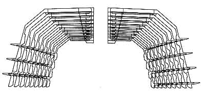
3.1.7. Comparison between the Zweymüller SL stem and the straight Müller stem
Here is an example of the straight Müller stem drawn without growth factors: the length of the metal neck is constant for all sizes, the head is fixed and the Operator has no means of compensating for residual differences in joint tension after hardening cement.
On the variants and numerous copies of Müller's self-locking prostheses, with interchangeable heads, the constant length of the metal neck was too long for the small sizes and too short for the large ones.
The short, medium and long necks of the modular heads are used to compensate for the lack of neck variation and are therefore no longer available for the latest joint tension corrections.
In my concept, applied to the Zweymüller prostheses, the metal necks vary regularly and the availability of heads with short, medium and long necks must be reserved to compensate for residual variations in joint tension.
----