3.2. The Method of Optimized Sizes
3.2.1. Summary
This method makes it possible to eliminate the imperfection of the series of stems whose sizes are scaled linearly, where the gaps between the small sizes nevertheless remain large, and the gaps between the large sizes unnecessarily small. With an optimized series, a patient, whatever the size of their bones, receives the implant that best meets their needs.
3.2.2. Optimized Sizes
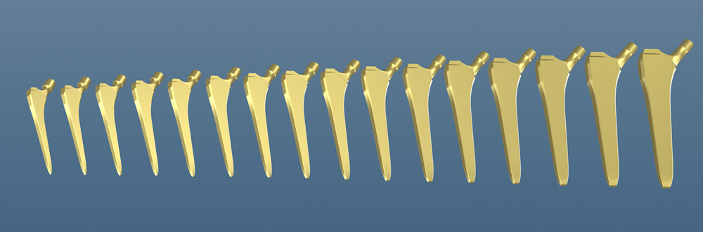
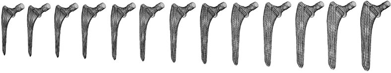
Optimized Sizes ensure, with a series of mass-produced implants, an optimal fit for each patient, with a limited number of sizes.
The variation between Optimized Sizes by the Growth Factors method is progressive. The small sizes are relatively close to each other and the large sizes have increasingly large gaps.
This method makes it possible to eliminate the imperfection of the series of stems whose sizes are scaled linearly, where the gaps between the small sizes nevertheless remain large, and the gaps between the large sizes unnecessarily small.
With an optimized series, a patient, whatever the size of their bones, receives the implant that best meets their needs. It is obvious that for a very small patient, both the preparation and the choice of the implant must be more precise than for a very large patient.
To guarantee consistency between the length and width of the stems and statistically satisfy the vast majority of patients, I mathematized the problem using the Growth Factors process, which allows the creation of series of Optimized Sizes.
By this method, the geometric relationships between the various areas of the implant remain preserved, and all sizes in the series satisfy all the laws of Geometric Anchoring.
3.2.3. Critic of non-optimized sizes
When the design of implants and sizes is manual or done using traditional drawing software, no relationship is formulated between the proportions of each implant.
No growth strategy is applied, except that each size grows in some areas, and sometimes even decreases in other areas.
3.2.4. Echelonnement régulier des Tailles Optimisées
My settings defining the distribution of sizes mainly take into account long experience of surgical assistance and not abstract considerations:
1. For the smallest and largest sizes, all the important criteria that we wish to take into account must be defined at the start of the design (length, width, thickness, neck length, etc.)
2. Then the number of sizes in the series is defined by the ideal admissible difference between each size so that the Operator has the possibility (for the hip for example) to position the top of the prosthesis, and therefore the center of the head, at the ideal height from an orthopedic point of view, and thus be able to reconstruct all the desirable total bone lengths with near continuity.
3. By exploiting the Ascending Interlocking property of the implants and having the possibility to adjust the grating depth, the Operator can reach any intermediate position.
Since the creation of my SL AlloClassic prosthesis in 1984, to my knowledge, no criticism of the gap between sizes, or of the absence of a missing intermediate size, has been expressed. I can therefore consider, with almost 40 years of hindsight, that the Optimized Sizes method has definitively resolved this problem.
3.2.5. Optimized Sizes and Gaussian Distribution
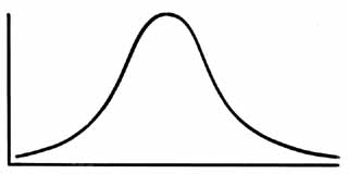
When we establish the histogram of the frequency of implantation of the sizes of a series of optimized implants, we obtain a Gaussian bell curve distribution.
This distribution according to a histogram in the shape of a Gaussian bell curve can be used to guide the stocking of sizes in the operating room, inventory management and manufacturing by producers.
3.2.6. Optimized Sizes meet rare exceptions
As with all mass-produced prostheses, prostheses whose sizes are optimized, while being statistically well adapted to all patients, present some limitations in 1 to 2% of cases.
The typical example (which I have actually observed) is the case of a young patient, around 40 years old, very active and rather tall. Its cortex is very thick and the diameter of the medullary canal is small. Therefore, this patient can only receive a small size stem from the optimized series. As neck lengths are also variable and statistically matched to patient sizes, the neck length this patient receives will be insufficient
However, these cases are predictable and plannable and several options remain available to the operator:
a) implant a size larger because the series of implants has the property of Ascending Interlocking, and decide to grate longer to implant a larger size. The design of the rasps still allows medullary canal preparation to continue (10 rasping cycles). This is the attitude I recommend.
b) use, exceptionally, a head with an extra long neck
c) implant the acetabulum less deeply or use a lateralized insert
For these particular cases, if these options are not suitable, the Optimized Sizes series does not compete with custom-made implants.
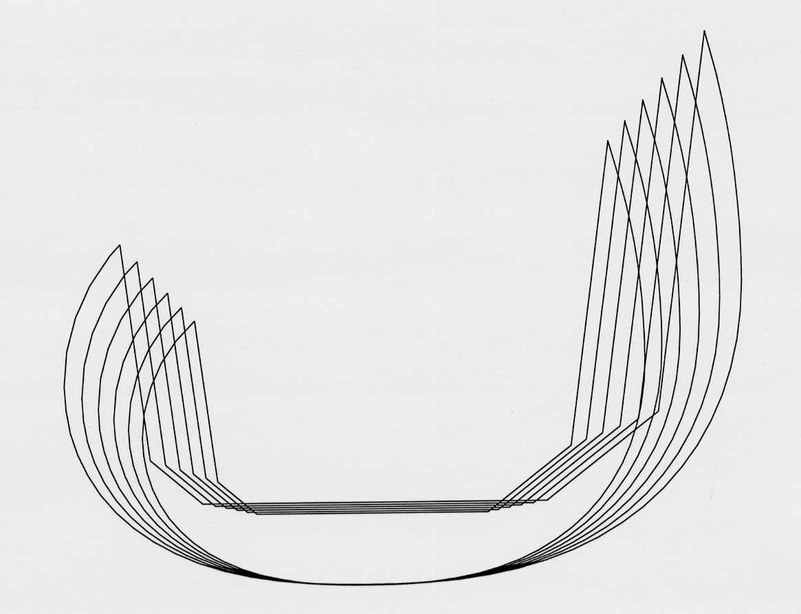
3.2.7. Application of the Optimized Size Method to the cups
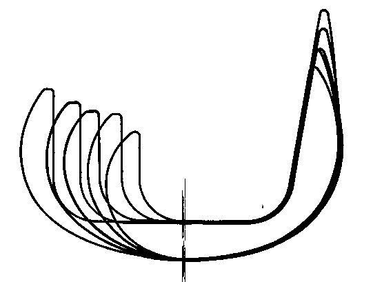
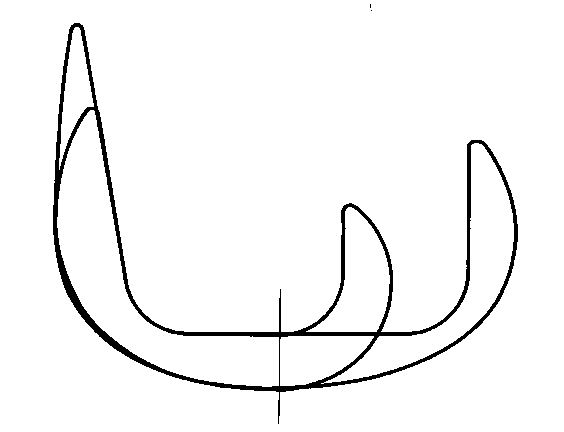
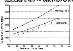
The concept of Optimized Sizes also has great importance in the design of cups. Indeed, Zweymüller's 1986 cementless screw-retained cups presented a very irregular distribution of dimensions.
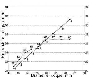
I solved this problem with the Bicon Plus cup from 1992, the 9 cup sizes of which are calculated by applying the principle of Optimized Sizes using the mathematical process of Growth Factors.
From one size to the next, the main diameters and the total depth of the shellcup vary with an increase independent of each other. Very small shells have a deeper and more "spherical" conformation, and large shells appear more flattened, or more "elliptical".
Il ne s’agit en aucun cas d’une croissance homothétique où toutes les dimensions varieraient avec le même facteur.
3.2.8. History of the Optimized Sizes process
During my participation by Carl Zeiss in 1965 in research work on the combustion speed of powder rockets, I was able to realize the importance of the method of classification of grains, particles or objects when we must study their statistical distribution.
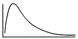
With a histogram subdivided into linear classes, no conclusions could be obtained.
With a histogram subdivided into logarithmic classes, on the other hand, the grains of powder (resembling small hollow macaroni) could be classified by their size as well as by their combustion surface, and positive conclusions could be drawn.
Ten years later, in 1974, also at Carl Zeiss, I again had the opportunity to see the advantages of the logarithmic histogram over the linear histogram. At the Bone Disease Research Institute, Institut Calot in Berck-Plage, I participated in a study on osteoporosis and the effectiveness of its treatments, such as calcitonin for example.
For this study, I installed a large research microscope connected to the Carl Zeiss "Microvideomat" image analyzer and a computer for which I carried out the theoretical part and all the programming, still in "machine language" at the time.
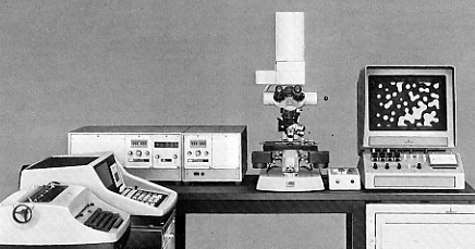
The study involved measuring the surface area of bone cells on thin, polished sections of biopsies. I had programmed the presentation of the measurement results in the form of histograms on a thousand cells per patient, with not linear but logarithmic classes.
As the Standard Deviations of the cell populations were of the same order of magnitude as the differences to be observed on the histograms, before or after treatment, only the logarithmic classification made it possible to concretely observe the results.
The transposition of these mathematical reflections to series of prostheses was not easy. Paradoxically, it is the sizes of prostheses that constitute the classes into which patients are distributed. It is the patients, and in the example of the hip, the shapes and dimensions of the medullary cavity of the proximal part of their femur which constitute the population to be classified in histogram.
----