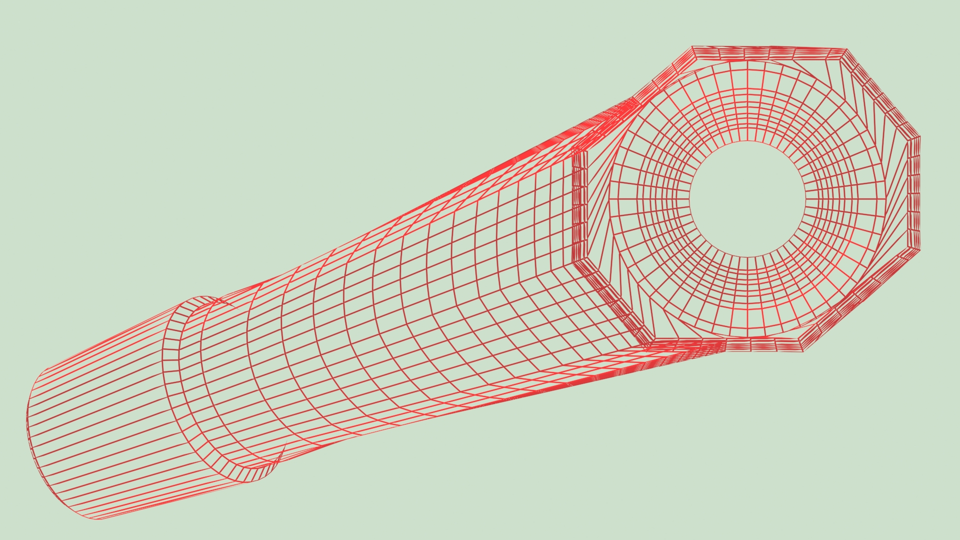
3.6. The Transition Curves
3.6.1. Summary
This is a set of different modeling procedures to optimize for example the transition between the proximal portion of a femoral stem and the upper part of the femoral neck replacing the traditional circular arcs.
According to the zone considered on the implants, the search of the best mechanical resistance taking into account the metal and its treatment, the needs related to the limitation of space available in the osseous beds, the precautions to take to avoid the contacts prejudicial between moving components, the models of Transition Curves can be very different.
Finally the search for Transition Curves could be gradually wide in the future with the modeling of the increasingly complex trajectories of the osseous trabeculae.
I carried out several incursions into this field by introducing nonplane trajectories into certain projects of prostheses designed to be with more close to the anatomy.
3.6.2. The search of better modelings
In my successive searches to seek the ideal curves of transition between the direction from the axis of a femoral stem and the direction of the neck, I had the opportunity to implement several mathematical modelings.
Until there and almost without exception in mechanical engineering, one passed from a direction to another by using an arc of circle to avoid the embrittlement of one part at the place of the change of direction. That is perfectly appropriate as long as there is no additional requirement on the drawing of the machine element, such as for example limitations of place or weight or conflict with another part. Even in aeronautics, if a part is not sufficiently solid, just make it bigger and heavier!
On the other hand, for the orthopedic implants, the place in the bone of the patient being limited, it is difficult to implant a size bigger than its medullary cavity.
3.6.3. Transition Curves and finite elements method
The method of the analysis by” Finite elements” of the constraints undergone by mechanical elements is frequently used to test the implants drawn by a CAD software. I learned this method by following the courses of Professors Lavaste and Landjerit to the School of Arts and Metiers of Paris.
This method makes it possible to simulate the constraints undergone by a mechanical element and to highlight the zones where the part will be overloaded and will be likely to break. Then, the part is corrected or redrawn, ( without calculations ), and one applies the method again to know if the corrections were advantageous. For example, one increases a little the radius of the arcs of circle of transition.
It is a method of validation a posteriori of an already finished drawing. The method requires important means of computing and, while being computerized, utilizes many roughly definite and perfectly subjective parameters by the operator.
The study by the method of the ”finite elements”, of a three-dimensional object requires to cut out this object in small elementary volumes, for example tetrahedra, whose sides are neither very small, nor infinitely smalls, but of known, measurable and calculable” finished” size. This cutting in small elementary volumes (“discretization”) is often automated by the software, and in this case the grid obtained is abundant, but disordered and obeys especially choices of density or dimensions. On the other hand, it is also possible to define the nodes of the grid manually, which is particularly hard. Only one minimum of points are collected and the precision of the results is lower.
Often, one gives up the three-dimensional grid to study the object only out of plane cut. One extrapolates the results with the third dimension by logical deduction, but by taking the risk of big mistakes. An example was the comparative analysis of the stems of Zweymüller first generation by HUISKES . This procedure occulted the third dimension which is however at the origin of the clinical superiority of the Zweymüller stems.
My philosophy is rather to anticipate, by the reflection and the theory, the results which one would obtain in a foreseeable way with the finite element method. For the various zones of the implants, I sought favorable and programmable mathematical modelings.
That makes it possible not to undergo the too strong approximations of the finite element method. A control by the finite elements is always interesting thereafter.
3.6.4. The catenary curve
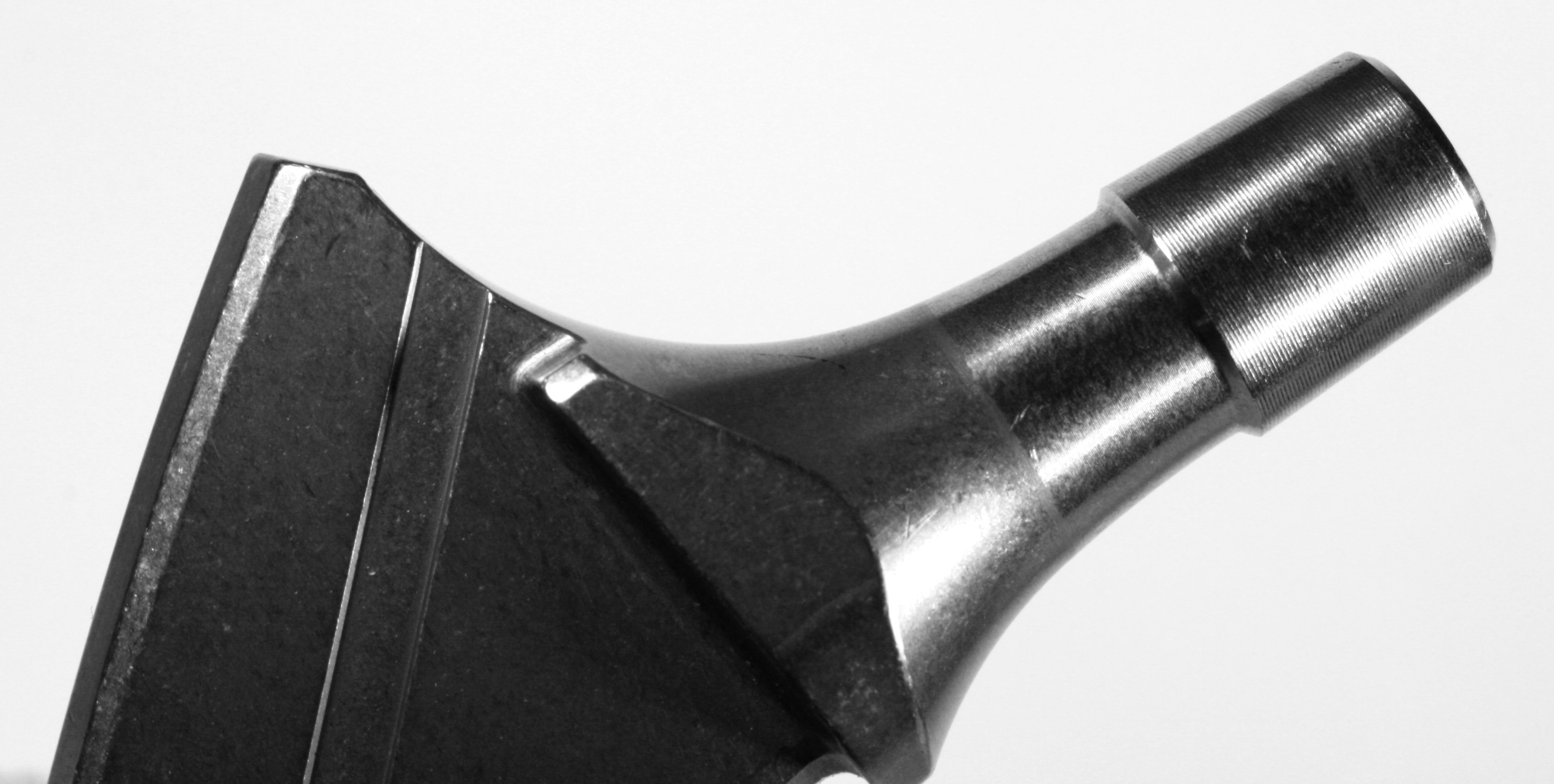
In a hip prosthesis, the intertrochanteric region, between the top of the proximal stem and the neck is an area where the metal is always subjected to tensile stress by the constraints from the head. It should be noticed that the prostheses with intramedullary stem differ from the reality of the architecture of the natural femur because the great trochanter, which was initially related to the natural neck, is not related any more to the prosthetic neck, and a small edging which I rather allot to the elastic movements of the great trochanter that with the movements of the stem in the diaphyse can be observed. The exception is the example of the old stems known as” isoelastic” of Robert Mathys, where it was necessary to connect the trochanter to the stem by a screw of traction to try to compensate for his hyperelasticity.
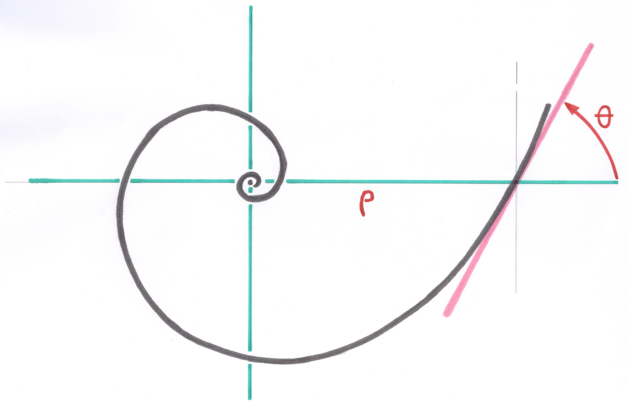
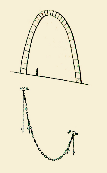
A way of modelling this area is to imagine (without really doing it) in this zone a ”discretization” by layers, i.e. by the theoretical cutting of the object initially in successive layers as the the layers of an onion, and then by the cutting of each layer by a meshing. Each layer considered independently would behave as if it were subjected to a traction as a tended skin, while actually remaining adherent with the subjacent metal mass. This way, each layer would take in an ideal way the shape of a catenary curve. The catenary curve isthe form taken naturally by the chain of a collar, on the one hand because of gravity on each link of constant mass, and on the other hand of the obvious constancy of the tension in each point all along the chain.
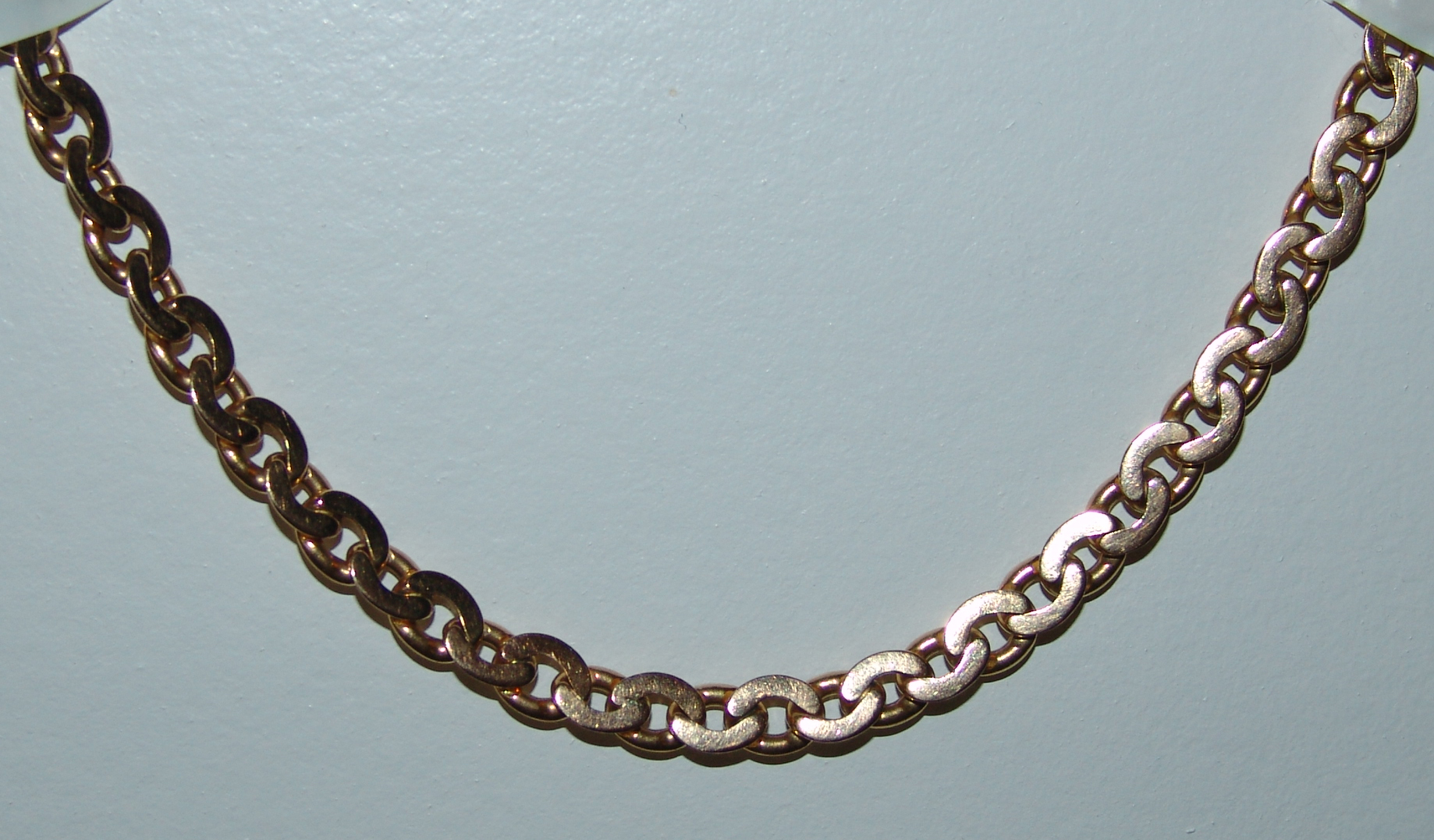
Because of this analogy, one calls commonly “catenary curve”, the plane curve followed mathematically by the Hyperbolic Cosine of the form Y = CH X . with CH X = ( e^x + e^-x ) /2 or the series form I used: CH X = 1 + X^2/2! + X^4/4! + X^6/6! + X^8/8! + X^10/10! + etc...
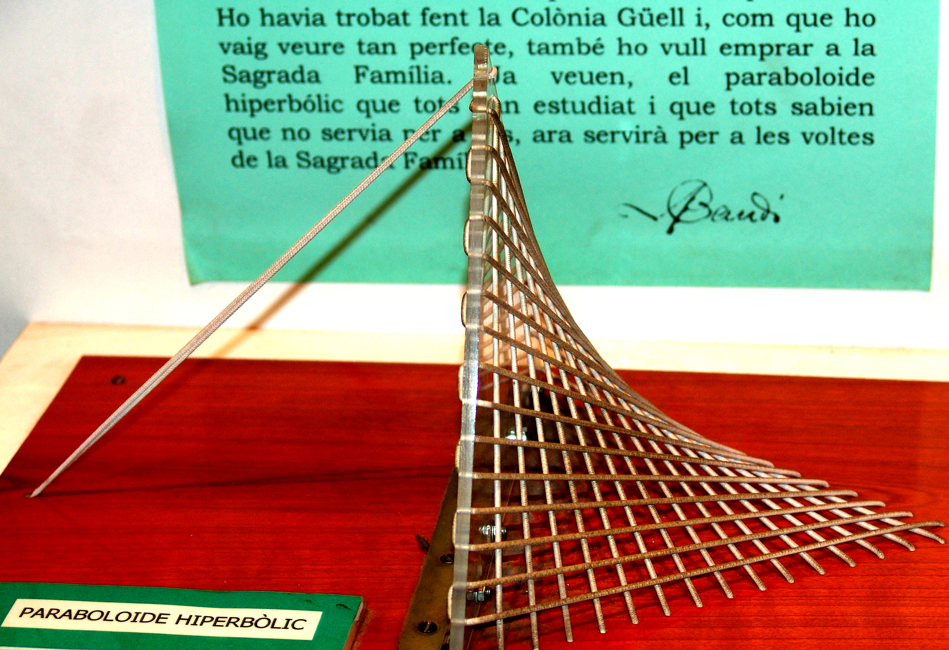
3.6.5. Rencontre with Gaudi... one century after
Recently, in 1999, whereas the majority of my projects of prostheses were finished for a long time, I took note of the astonishing works of Antoni Gaudi (1852 - 1926). My satisfaction came from the great analogy of its thought process to treat the transition curves, which I had adopted for 25 years to design the curves and surfaces of transition in the implants. For a long time I was impassioned by the families of curves passing gradually from the angular forms to round forms, which I called here Transition Curves.
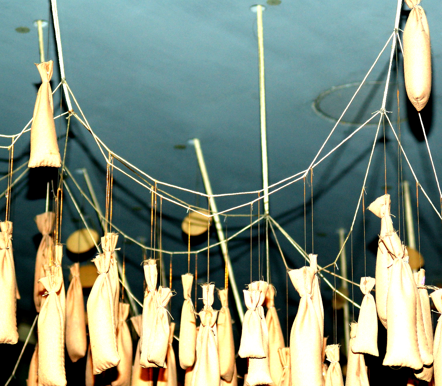
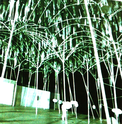
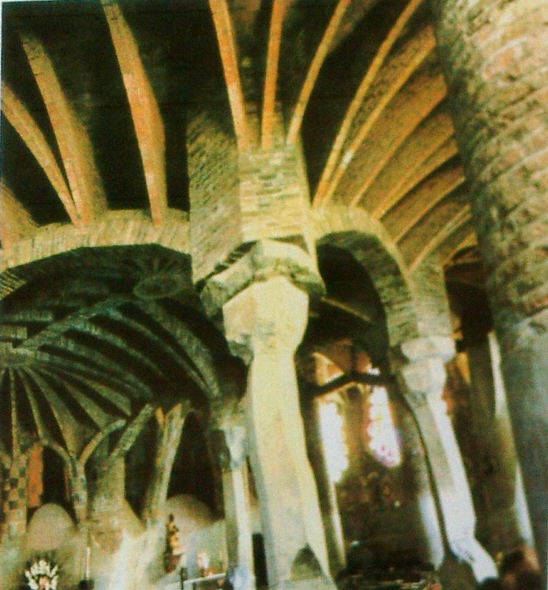
The famous architect of Barcelona, Antoni Gaudi, had the fabulous intuition to draw the plans of the cathedral of Barcelona and the vaults of many buildings by regaining exactly the shapes of chain taken naturally by his models consisting of fine suspended cords hanging upside down the ceiling of his workshop.
3.6.6. Gaudi Geometry researcher
In the workshop next to his office, Gaudi developed a real research program on aspects of geometry that could be important for his work as an Architect...
He focused on the experimental quest for optimal geometric solutions that he could apply to his projects. Curvatures, surfaces and transformations only interested him if he could apply them in his constructions. ... He created a geometric universe to serve his own creativity. (Claudi Alsina i Català, Mark Burry, Gaudi Unseen, Jovis Berlin.)
If the other builders of cathedrals had had the intuitions of Gaudi, hundreds of buildings would currently not be pile of ruins.
For several families of implants, I chose this catenary modeling of the zone where metal is requested in traction, by introducing the coordinates, calculated in advance by the Hyperbolic Cosinus function, in the parameters describig the intertrochanteric transition curve until the base from the conical junction with the head.
3.6.7. The hyperbolic transition curve
To model the transition between the anchoring zone and the cylindrical neck from the stem AlloClassic (1984), not wanting to apply a curve of transition in arc of circle which I found too bulky, I researched a curve leaving very gradually the anchoring zone and whose curve varied regularly to reach tangentially the base of the cylindrical neck.
My application of the hyperbolic transition to the family of the AlloClassic stems was the subject of my patent…. (6.2.6. ).
Thanks to its transition curve in the shape of hyperbole arc, the AlloClassic stem entered very rarely in conflict with the calcar in the vicinity of the cut of the neck. This form was criticized because the filling and the contact with the osseous bed in this area did not seem sufficient with the eyes of some, at least on the X-rays of face.
Thanks to Geometric Anchoring, the AlloClassic stem however is sufficiently stabilized by its anchoring zone, and I estimate today that it was not essential that the métaphysary filling be more complete. It was statistically very interesting, for the correct use of the Impaction Reserve, to make rare the conflicts which would have prevented 4 or 5 millimeters of additional impaction.
3.6.8. The exponential transition curves
Radiologically, the AlloClassic stem remaining sometimes without apparent contact with the calcar, during the creation of stem SL Plus, it was required of me to increase the filling of the zone of the calcar.
For stem SL Plus, I adopted a mathematical modeling of the transition curve whose variation of the radius of curvature along the arc of transition could be parameterized more easily, whereas for the hyperbolic model of the AlloClassic stem, the maximum curvature was always at the base of the cylindrical neck.
Modeling by a portion of exponential curve defined in a not orthonormed local frame of reference, (see 4.3.2. ), has as an advantage of having a perfect tangency with the anchoring zone in its starting point and allows to satisfy my Law of the Positive and continuous Derivates, more rigorously than with the hyperbole.
This modeling also allows setting continuous the angle of the tangent to the curve at the point of arrival at the base of the junction cone. This modeling completely replaces the cylindrical part of the neck. In practice, the parameters of this curve are calculated automatically for each size by an algorithm by successive iterations.
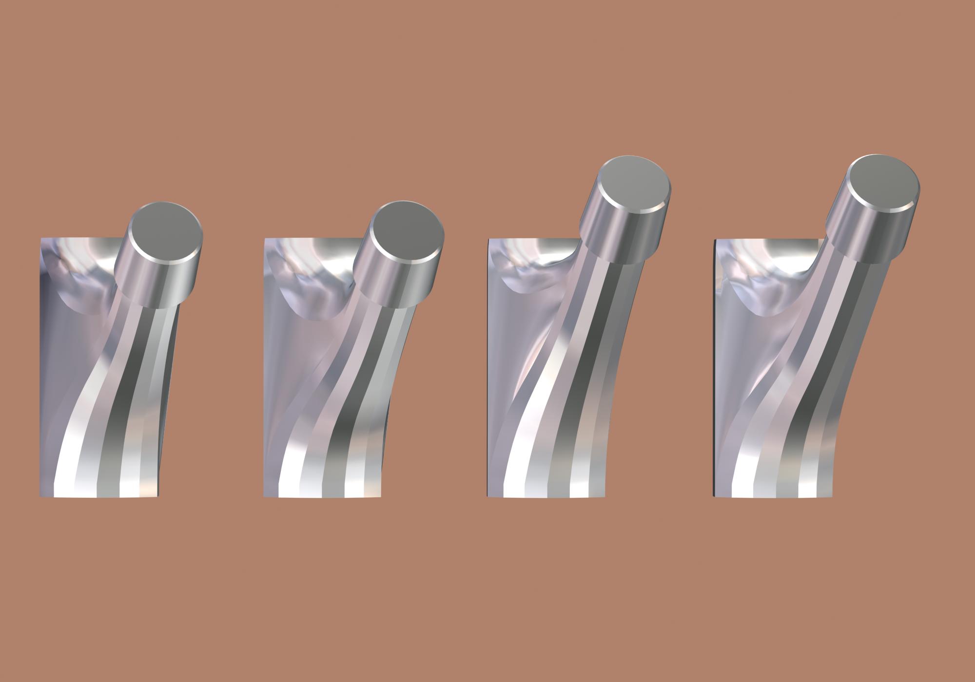
3.6.9. The method of missile launches in the plan
For the modeling of the proximal parts of the system Modular Plus, I applied a method of automatic calculation. The symmetry left-right of these parts made it possible to describe each curve connecting the base of the proximal to the base of the cone junction, in a vertical plane. The surface connecting the medial part of the base part to the cone is composed of 24 successively calculated curves.
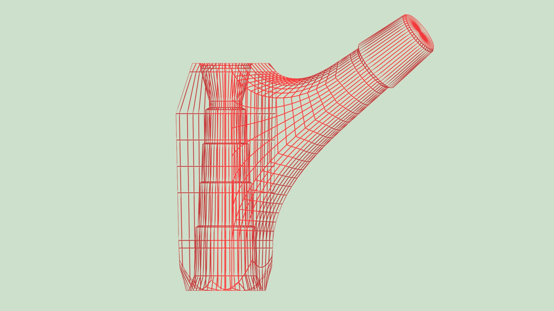
3.6.10. Method of three-dimensional shootings of missiles
For the modeling of the nonsymmetrical left-right proximal parts of the ANA.NOVA project, it was not possible any more to preserve the plane transition curves.
The new concept of the anterior shift of the axis of the neck, the implant still closer the actual anatomy of the proximal femur, required to connect stem and neck by three-dimensional transition curves.
This method performs an automatic simulation of the orientation lines of the crystalline components of cortical bone and the orientation of the bone trabeculae of cancellous bone, close to the orientation of real constraints.
The generation of these transition curves is a model similar to the trajectories of homing missiles pursuing a moving target, not remaining in the vertical plane of the launch.
To be a little more explicit, the path from the stem to the base of the cone is divided into a number of segments. By an automatic iteration of the algorithm, the successive segments are partially deflected in 3D towards the target, to end up with the last segment to be aligned with the targeted segment on the periphery of the cone, and this on 24 different trajectories in 3D.
----
Next chapter: 4. Specific methods for femoral stems