5.4. Knee DECKNER -GF, project
( Growing Factors ) , project
5.4.1. Subject of the research
The search for a geometry with high clearance and simultaneously self-stabilizing properties was the basis for the development of this new knee prosthesis.
After achieving great success with the GSB knee prosthesis as director of the French subsidiary of AlloPro (1978-1992), and having participated in over 600 initial knee implants and 1,400 hip implants, including the preliminary preparation of orthopedic surgeons, I gained the necessary experience for the development of new implants. My training as an engineer, computer scientist, and nurse allowed me to lead the development of this knee from the initial design phase to the production-ready digital files.
The search for sliding surface pairs with the properties of natural return to the extension position, anteroposterior, and medial-lateral refocusing led me to the following results:
5.4.2. The anteroposterior contour of the femur
The anteroposterior contour of the femur should no longer be a collection of successive circular arcs, but should include a curvature that varies continuously with very little curvature in the direction of extension.
This curve can be obtained in computer codes by evolving circular arcs by applying real, non-integer, powers to their trigonometric components.
Condylar curvature varying continuously with representation of the radii of curvature calculated at each point
5.4.3. The frontal section of the femur
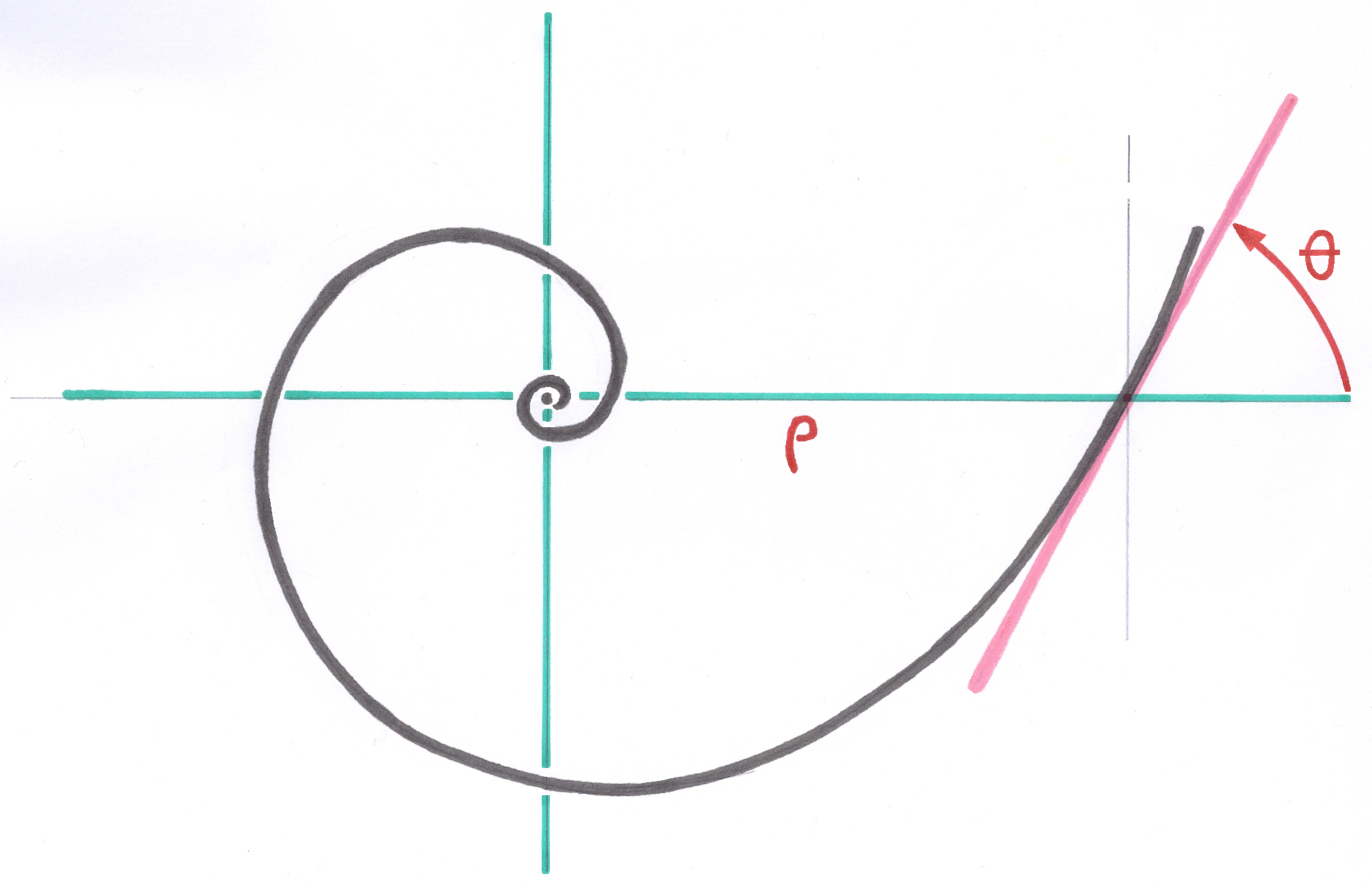
It is this "frontal section" that presents the greatest innovation in this knee prosthesis. The ideal formulation of this curve appeared to me while observing the greater stability of a ball at the bottom of a spherical bowl with a radius slightly greater than the radius of the ball. The return toward the center increases rapidly as the ball moves away from the center of the bowl due to the increase in the slope between the two neighboring surfaces. However, the closer one gets to the lowest point of the bowl, the more the movement remains relatively free. The potential energy is lowest when the ball is at the bottom of the bowl. In a knee fitted with a total knee replacement, this potential energy is represented by the tension of all the ligaments (those left in place after surgery or illness). This energy is minimal when the ligaments are relaxed and the knee is in the resting position, i.e., centered and extended.
First representation of the sliding surface
5.4.4. Cycloidal Wave Geometry
The ideal shape of this curve is that of a wave in the open ocean or a deep-water swell (such as the Gerstner swell). The Cycloidal Wave (actually a hypocycloid or trochoid) is a curve generated by a point inside a circle rolling whithout gliding along a straight line. The general formula is:
x(t)=r(t-sin(t))
y(t)=r(1-cos(t)) to be completed by AD
Bibliography: Jacques Bouteloup, Waves, Tides, Marine Currents, PUF, 1950
H. Bouasse, Houles, Rides, Seiches et marées, Delagrave, 1924.
Gerstner Swell, Mathematical Formulas.
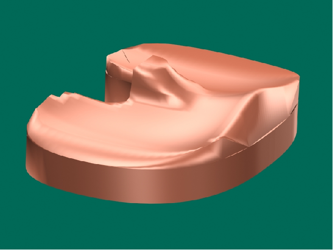
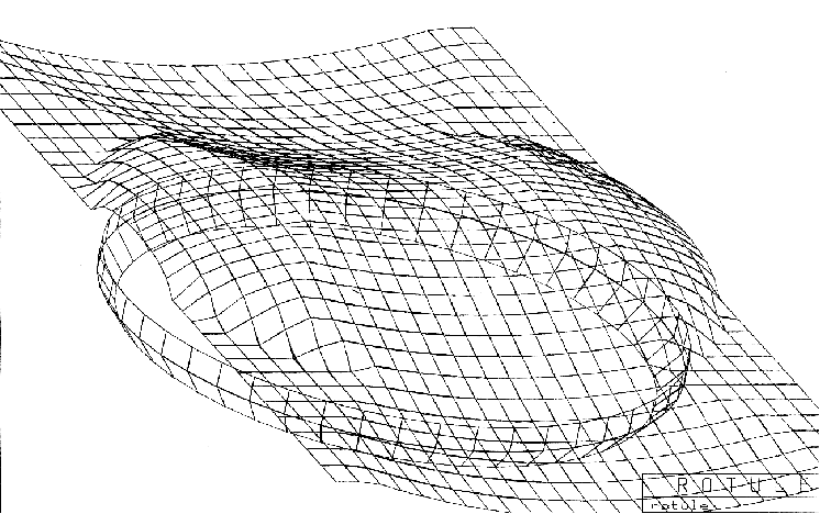
5.4.5. Composition of the Femur Sliding Surface
The Cycloidal Wave curve is projected by calculation at each point of the femoral condyle profile curve, perpendicular to each segment at each point. This produces a surface that closely approximates the natural surface of the femur, while still being achievable for finishing by profile grinding or digital rectification.
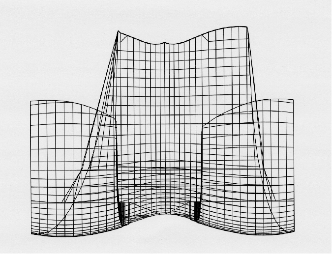
Cycloidal wave profile of the sliding surface Note the lateral and medial rise of the wave, which contributes to the automatic return to center facing the tibial plateau, which exhibits a similar rise.
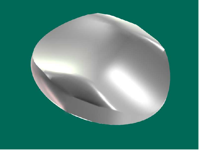
5.4.6. The patellar guidance shield is vertical
The path imposed on the patella is perfectly vertical, that is, perpendicular to the plane of the condyles. When observing the movements of the natural patella, they are vertical, except when the quadriceps is completely relaxed and the patellar ligament is loose, and a slight medial movement of the patella is observed. I believe this small movement can be ignored for the prosthesis, if the guidance is sufficient.
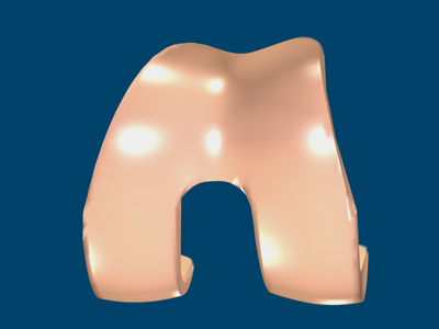
Ceramic femur sliding surface
5.4.7. The tibial prosthesis is also shaped like a Cycloidal Wave
The sliding surface of the tibial plateau is shaped like a Cycloidal Wave, with the sides slightly raised, like the lateral and medial continuation of the wave. Anteroposteriorly, the surface follows the same shape as the femur, slightly enlarged to allow slight free movements driven by the structure of the various knee ligaments, slightly modified by the surgery.
The gap between the femur and the tibia will be refined to allow each tibial plateau to accommodate a femoral implant one size smaller or larger than the nominal size.
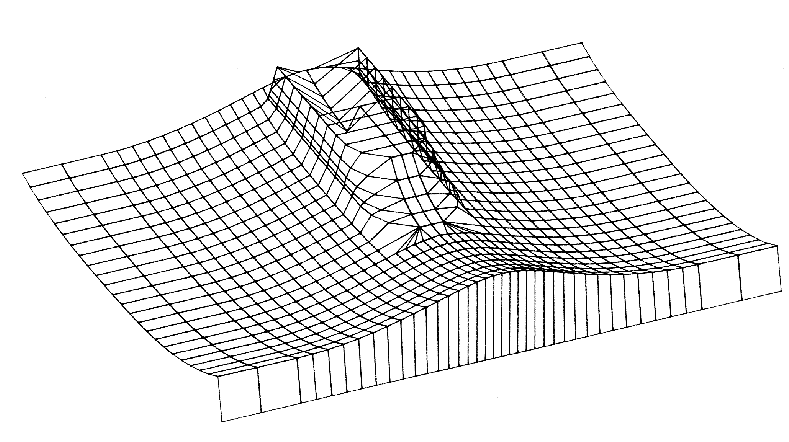
Sliding surface of the tibia with cycloidal wave profile
5.4.8. Central Tibia Guidance
A central stop limits the movement between the tibial plateau and the femoral implant. In particular, it allows for a certain degree of freedom of rotation, which spares this prosthesis the complexity of a mechanical rotation axis system. Moreover, implants that allow rotation therefore lack additional freedom of movement. These implants also lack multi-axial return geometry.
The central stop limits posterior deviation of the femur, but gently, with a natural return function thanks to the forward arc slope.
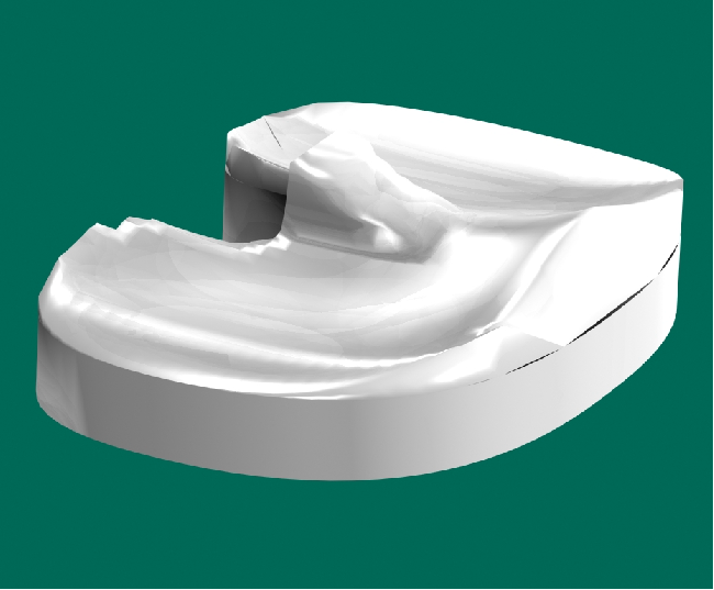
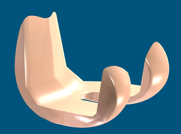
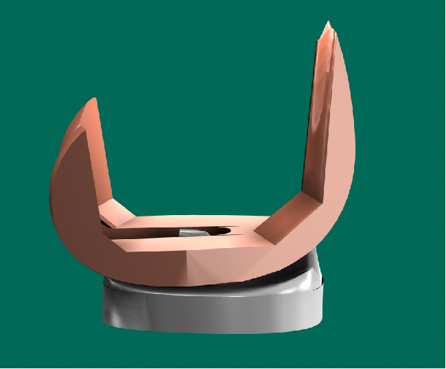
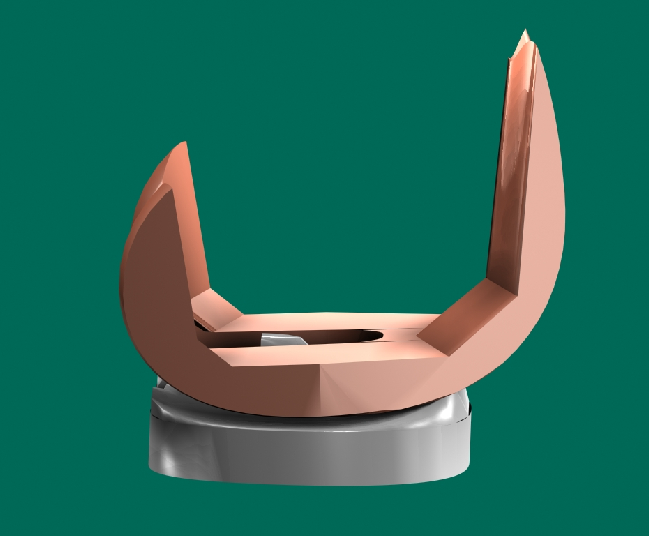
Computer-generated image of the polyethylene tibial plateau
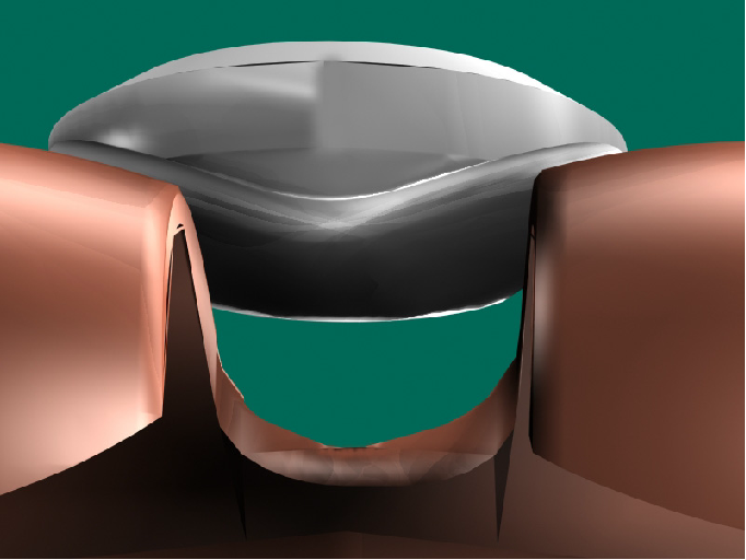
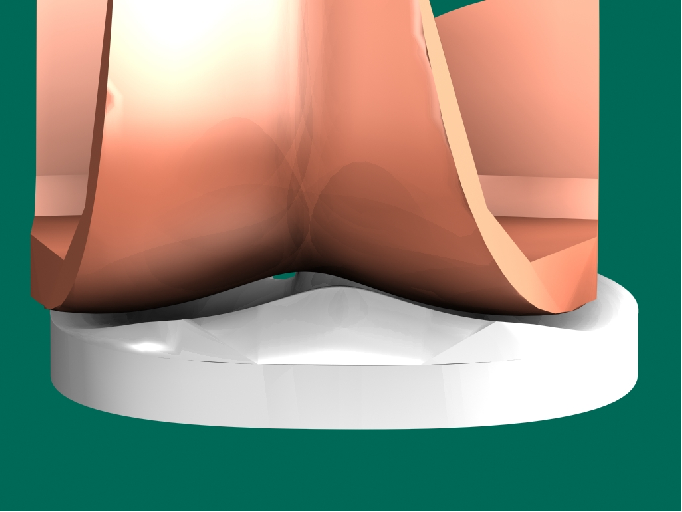
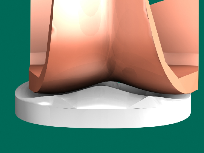
5.4.9. The posterior notch
This notch leaves a small space for any remaining cruciate ligament.
Computer-generated image of the ceramic tibial plateau
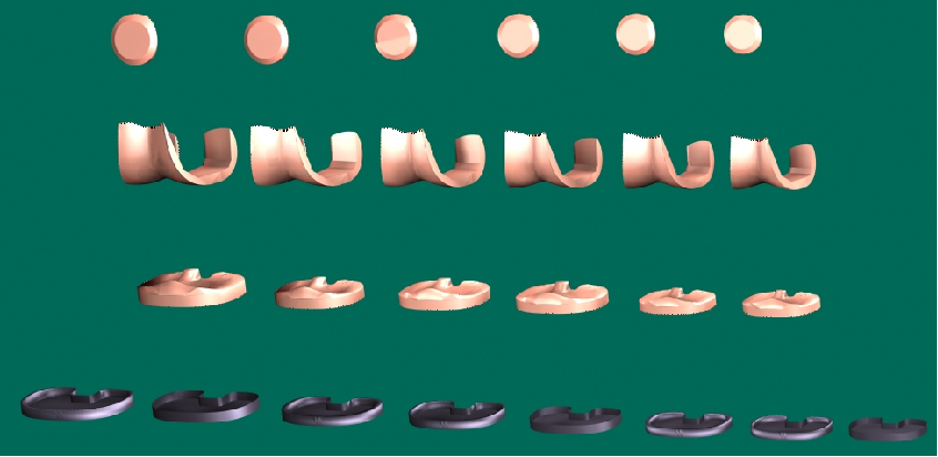
5.4.10. The patellar implant
The patellar implant has the same geometry as the femur and tibia, i.e., a cycloidal wave-shaped profile, very similar to that of the femoral implant. The sagittal curvature is a good compromise between the variable curvatures of the femur, made possible by the small size of this patellar implant.
Graphical representation of the cycloidal wave sliding surface of the patellar prosthesis
Computer-generated image of the polyethylene patellar prosthesis
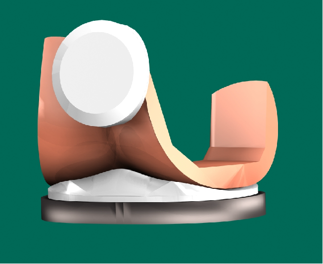
5.4.11. Patellar Implant Refocusing Effect
Due to the wavy design, which is very close to the real femur, and for relatively wide decenterings, the patella is re-centered.
The cycloidal wave profile automatically recenters the ball joint
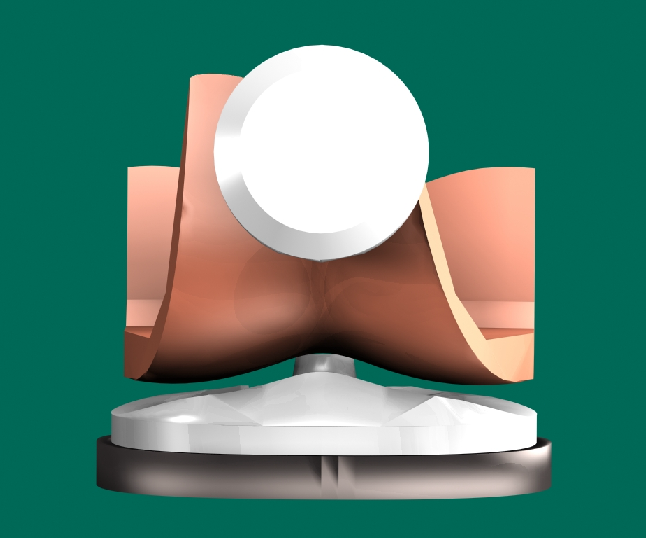
5.4.12. The patella remains guided.
For any degree of knee flexion, the patella remains centered in its groove.
Die Zentrierung erfolgt in jeder Position der Patella
Centering takes place until extreme flexion
5.4.13 Highly stable assembly of the femoral prosthesis on the bone
All junction planes between the already prepared femur and the femoral implant belong to the same geometrically exact cone, and all the generatrices of all fixation surfaces converge at the same point on the impaction axis. This is far from being the case for most current knee prostheses.
If the compression planes are not part of a cone, then the dynamic pressures and compressions during impaction are not evenly distributed, and the implant deviates from its planned theoretical position and can deflect and even crack a condyle.
The presence of fixation pins that are not aligned with the theoretical axis of the cone contributes to the degradation of the cancellous bone and hinders proper impaction. This was precisely the case with the old AlloPro prosthesis studied above, which was designed and not calculated.
In the current prosthesis design, these fixation pins or studs are no longer necessary. A slight surface structuring of the compression planes is essential. A small impaction reserve must also be provided (see Glossary 6.1.).
Graphical model of the conical junction with the femur bone
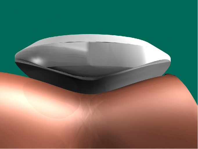
5.4.14.
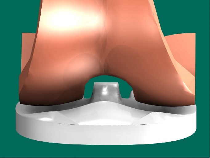
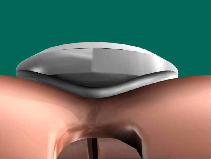
Example: polyethylene tibia and ceramic femur
5.4.15.
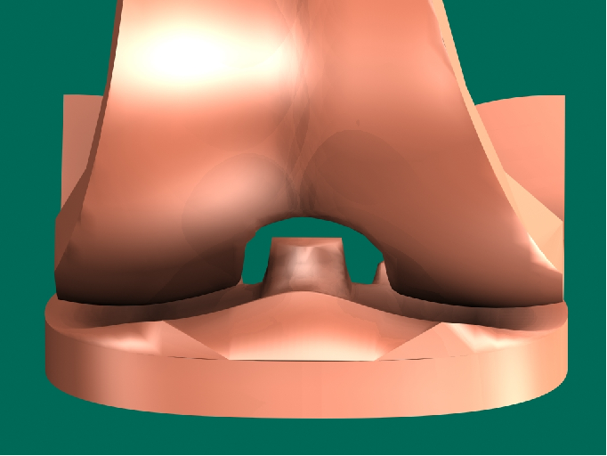
Possible example of ceramic tibia and femur
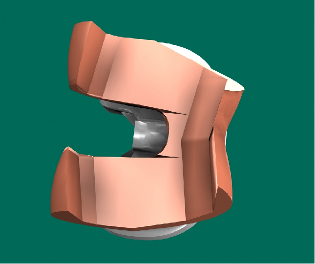
5.4.16.
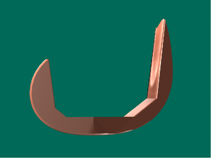
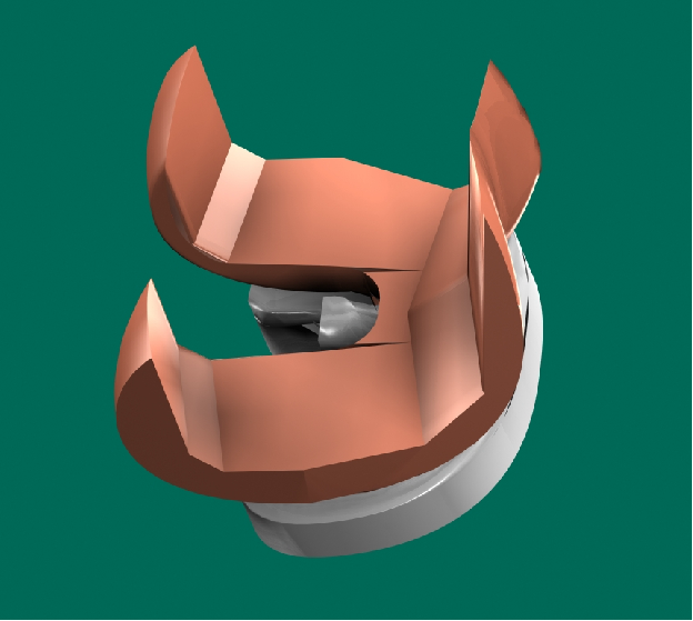
Lateral femoral prosthesis, the mathematically conical junction not requiring an additional fixation system
5.4.17.
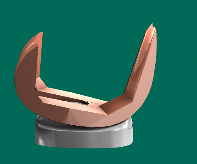
The system allows for a few degrees of hyperextension
5.4.18.
The slide allows a small "drawer" movement
5.4.19.
Due to the calculated radii of curvature, the prosthesis automatically seeks to recenter itself in anteroposterior direction, that is to say in perfect extension
5.4.20.
Thanks to the cycloidal wave profile, an automatic return to the center takes place after a slight medial shift of the tibia
5.4.21.
Return to the center after a small lateral shift of the tibia
5.4.22.
Automatic sagittal recall after internal or external rotation
5.4.23.
Vertical view of the rigorously calculated conical bone-prosthesis junction. The anteroposterior conical clamping planes are directed in the direction of each condyle, to avoid any risk of bone cracking.
5.4.24.
Polyethylene tibial sliding plate with titanium base (before representation of the essential tibial fixation system)
5.4.25.
Elevated view showing the recentering cycloidal wave
5.4.26.
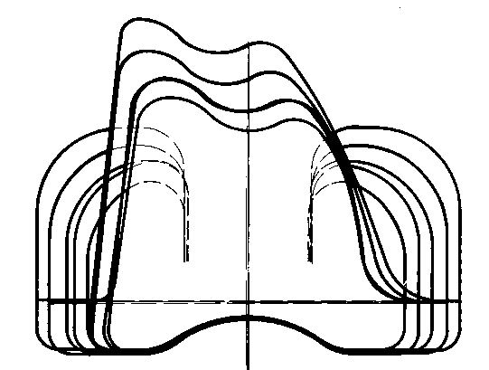
Superimposed femurs from the front of an old Allo Pro knee We observe a variation in the obliquity of the patellar guidance, a common distal glide pattern for all sizes, and uncontrolled variations in the anterior contour pattern.
5.4.27.
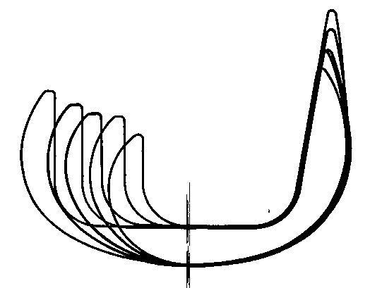
Side-on femurs of an old Allo Pro knee We observe a constant thickness at the base of the implants. The posterior bend of the smallest size has twice the thickness of the bend of the largest size. Only the anterior portion is inclined; the posterior portion is vertical. This is very far from a conical junction. In addition, the anchor rods, not shown here, cause a vertical descent. Fixation is impossible without damage.
5.4.28.
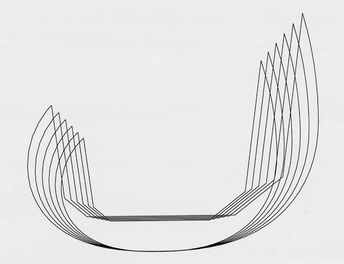
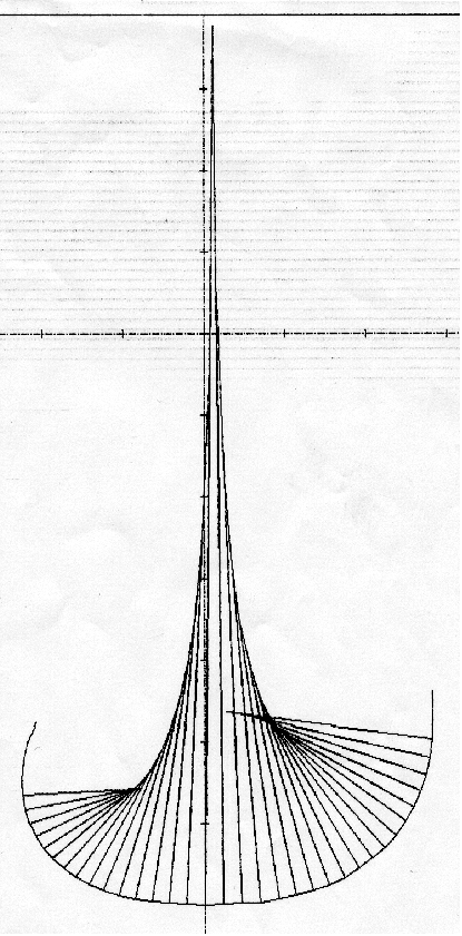
Lateral superimposed femurs of a DECKNER knee, in optimized sizes calculated using the growth factor method. In all directions, at all points, growth between sizes is regular and exponential in the mathematical sense. Distal thickness is slightly variable. The anterior and posterior bearing surfaces move apart simultaneously.
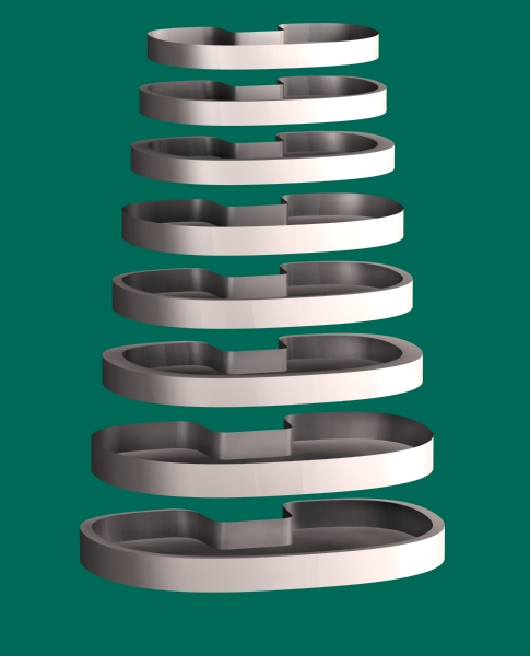
5.4.29.
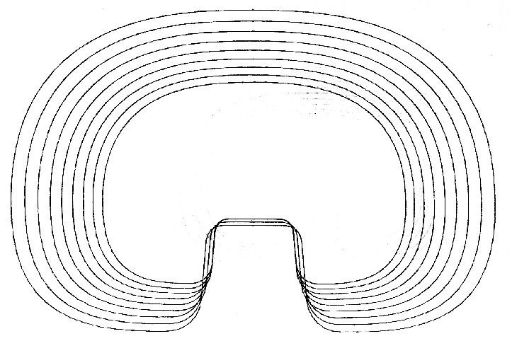
Contours of the tibial plateau bases calculated using the optimized size method. The height of the peripheries and the thickness of the metal of the bases are also variable, with independent Growth Factors.
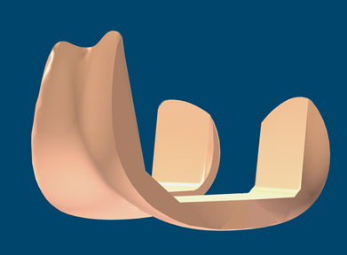
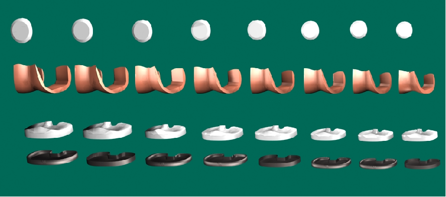
5.4.30.
The 7 bases only receive 3 tibial plates Example before representation of the tibial fixation system
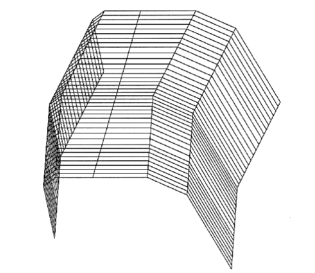
5.4.31.
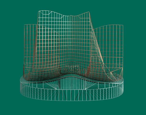
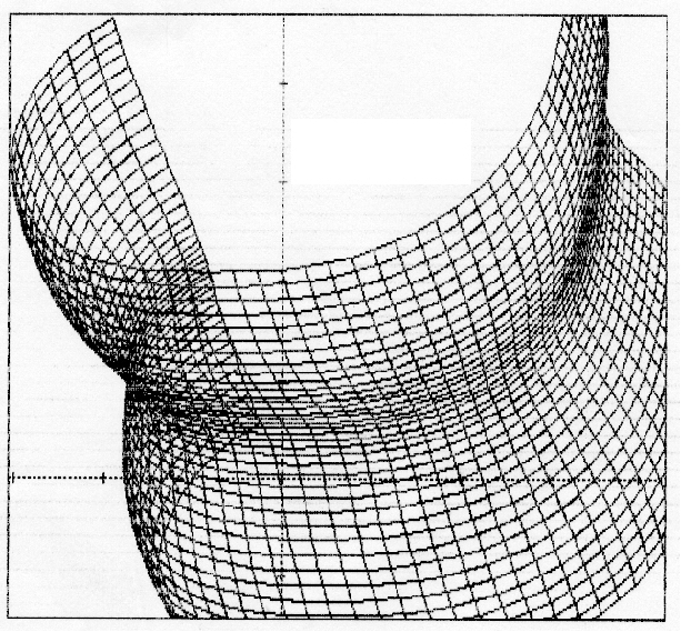
Front view in calculated mesh of the tibia-femur pair
5.4.32.
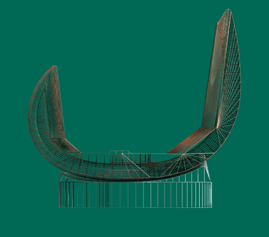
Side view of the calculated mesh of the tibia-femur pair
5.4.33.
Example of a complete system: 8 titanium tibial bases, three polyethylene tibial trays, 8 ceramic femoral parts, and 3 PE patellas
5.4.34.
Example of a complete system: 8 titanium tibial bases, three ceramic tibial trays, 8 ceramic femoral parts, and 3 PE patellas
----
Next Chapter: 5.5. Instruments